# now let's create a new column for seconds
# 1 second = 25 frames
gcs_sf_s = gcs_sf |>
  dplyr::mutate(sec = as.numeric(frame) / 25)

# group df by seconds
gcs_grouped = gcs_sf_s |>
  sf::st_drop_geometry() |> #drop geometry as it's not needed here
  dplyr::group_by(sec) |> # group by seconds
  dplyr::summarise(n = dplyr::n()) # summarise

gcs_grouped |>
head()4 Flow
Flow is one of the basic measures to quantify pedestrian dynamics (Steffen and Seyfried, 2010).
Flow is measured by counting the heads that pass through a line, e.g. doors, within a given time interval.
In this chapter we will find out three types of flow in Grand Central Station (GCS) and JuPedSim (JPS) model:
- Global, or the entire environment, flow
- Divided flow, which refers to the environment being divided into four equal polygons and measuring flow in each
- Selected flow refers to two manually defined areas – Zone 1 and Zone 2. Zone 1 has the density that is similar to that of the entire environment and Zone 2 has the highest density in the environment. For more information see chapter “Environment”.
4.1 1.1 Global flow (GCS)
4.1.1 Plotting
gcs_flow_plot = ggplot2::ggplot(gcs_grouped) +
  ggplot2::aes(x = sec,
               y = n) +
  ggplot2::geom_line()
We could add add additional information by adding lines indicating mean and median for seconds and number of agents, but I’m not sure it tells us much…
# let's calculate mean and median values of n to add to the plot
gcs_mean_s = gcs_sf_s$sec |> mean()
gcs_median_s = gcs_sf_s$sec |> median()
gcs_mean_n = gcs_grouped$n |> mean()
gcs_median_n = gcs_grouped$n |> median()

ggplot2::ggplot(gcs_grouped) +
  ggplot2::aes(x = sec,
               y = n) +
  ggplot2::geom_line() +
  ggplot2::geom_vline(xintercept = gcs_mean_s,
                      col = "red") +
  ggplot2::geom_text(ggplot2::aes(x=gcs_mean_s+5, label=paste0("Mean\n",round(gcs_mean_s,2)), y=80)) +
  ggplot2::geom_vline(xintercept = gcs_median_s,
                      col = "blue") +
  ggplot2::geom_hline(yintercept = gcs_mean_n,
                      col = "red") +
  ggplot2::geom_hline(yintercept = gcs_median_n,
                      col = "blue")
4.2 2.1 Divided flow (GCS)
# first create a list to store our multiple dataframes
gcs_joined = list()
for (i in 1:lengths(gcs_div_sf)){
  gcs_joined[[i]] = gcs_sf_s[gcs_div_sf[i,], op = sf::st_intersects] # all intersecting points will be selected
}

# sanity check
gcs_joined1 = gcs_sf_s[gcs_div_sf[1,], op = sf::st_intersects]
gcs_joined2 = gcs_sf_s[gcs_div_sf[2,], op = sf::st_intersects]
identical(gcs_joined1, gcs_joined[[1]]) # TRUE
identical(gcs_joined2, gcs_joined[[2]]) # TRUE
# group each sf object by seconds and make a list out of them
gcs_joined_grouped = list()
for (i in 1:length(gcs_joined)){
gcs_joined_grouped[[i]] = gcs_joined[[i]] |>
sf::st_drop_geometry() |>
dplyr::group_by(sec) |>
dplyr::summarise(n = dplyr::n())
}
# sanity check comparison (alert: ugly code!)
identical(gcs_joined_grouped[[1]], # first list of a list that was just made
gcs_joined[[1]] |> # repeating the same code as in the loop above but only on 1 (the first) list
sf::st_drop_geometry() |>
dplyr::group_by(sec) |>
dplyr::summarise(n = dplyr::n()))4.2.1 Plotting
In the plot showing flow in the entire GCS environment, I added means and medians but this time I will exclude them as I do not know if it’s valuable to have them at this stage. Plus, it will make the code shorter.
# let's create a list of plots showing flow in each polygon
gcs_flow_div_plots = list()
for (i in 1:length(gcs_joined_grouped)){
  gcs_flow_div_plots[[i]] = ggplot2::ggplot(gcs_joined_grouped[[i]]) +
    ggplot2::aes(x = sec,
                 y = n) +
    ggplot2::geom_line()
  # print(gcs_flow_div_plots)
}
# let's plot a polygons 1-4
gridExtra::grid.arrange(gcs_flow_div_plots[[1]], gcs_flow_div_plots[[2]],gcs_flow_div_plots[[3]],gcs_flow_div_plots[[4]], layout_matrix = rbind(c(1,2),c(3,4)))4.3 3.1 Selected (GCS)
# a list to store our 2 dataframes for the selected areas
gcs_joined_zones = list()
for (i in 1:length(zones)){
  gcs_joined_zones[[i]] = gcs_sf_s[zones[[i]], op = sf::st_intersects] # all intersecting points will be selected
}

# sanity check
gcs_joined_zones1 = gcs_sf_s[zones[[1]], op = sf::st_intersects]
identical(gcs_joined_zones1, gcs_joined_zones[[1]]) # TRUE
# group each sf object by seconds and make a list out of them
gcs_joined_grouped_zones = list()
for (i in 1:length(gcs_joined_zones)){
gcs_joined_grouped_zones[[i]] = gcs_joined_zones[[i]] |>
sf::st_drop_geometry() |>
dplyr::group_by(sec) |>
dplyr::summarise(n = dplyr::n())
}
# sanity check comparison (alert: ugly code!)
identical(gcs_joined_grouped_zones[[1]], # first list of a list that was just made
gcs_joined_zones[[1]] |> # repeating the same code as in the loop above but only on 1 (the first) list
sf::st_drop_geometry() |>
dplyr::group_by(sec) |>
dplyr::summarise(n = dplyr::n()))4.3.1 Plotting
# let's create a list of plots showing flow in each polygon
gcs_flow_zones_plots = list()
for (i in 1:length(gcs_joined_grouped_zones)){
  gcs_flow_zones_plots[[i]] = ggplot2::ggplot(gcs_joined_grouped_zones[[i]]) +
    ggplot2::aes(x = sec,
                 y = n) +
    ggplot2::geom_line()
  # print(gcs_flow_zones_plots )
}

gridExtra::grid.arrange(gcs_flow_zones_plots[[1]], gcs_flow_zones_plots[[2]], layout_matrix = rbind(c(1,2),c(3,4)))
4.4 1.2 Global (JPS)
# now let's create a new column for seconds
# 1 second = 25 frames
jps_s = traj1_sf |>
  dplyr::mutate(sec = FR / 25)

# group df by seconds
jps_grouped = jps_s |>
  sf::st_drop_geometry() |> #drop geometry as it's not needed here
  dplyr::group_by(sec) |> # group by seconds
  dplyr::summarise(n = dplyr::n()) # summarise

jps_grouped |>
  head()
4.4.1 Plotting
jps_flow_plot = ggplot2::ggplot(jps_grouped) +
  ggplot2::aes(x = sec,
               y = n) +
  ggplot2::geom_line()
jps_flow_plot
4.5 2.2 Divided flow (JPS)
# first create a list to store our multiple dataframes
jps_joined = list()
for (i in 1:lengths(gcs_div_sf)){
  jps_joined[[i]] = jps_s[gcs_div_sf[i,], op = sf::st_intersects] # all intersecting points will be selected
}

# sanity check
jps_joined1 = jps_s[gcs_div_sf[1,], op = sf::st_intersects]
identical(jps_joined1, jps_joined[[1]]) # TRUE
# group each sf object by seconds and make a list out of them
jps_joined_grouped = list()
for (i in 1:length(jps_joined)){
jps_joined_grouped[[i]] = jps_joined[[i]] |>
sf::st_drop_geometry() |>
dplyr::group_by(sec) |>
dplyr::summarise(n = dplyr::n())
}
# sanity check comparison (alert: ugly code!)
identical(jps_joined_grouped[[1]], # first list of a list that was just made
jps_joined[[1]] |> # repeating the same code as in the loop above but only on 1 (the first) list
sf::st_drop_geometry() |>
dplyr::group_by(sec) |>
dplyr::summarise(n = dplyr::n()))4.5.1 Plotting
# let's create a list of plots showing flow in each polygon
jps_flow_div_plots = list()
for (i in 1:length(jps_joined_grouped)){
  jps_flow_div_plots[[i]] = ggplot2::ggplot(jps_joined_grouped[[i]]) +
    ggplot2::aes(x = sec,
                 y = n) +
    ggplot2::geom_line()
  # print(gcs_flow_div_plots)
}
# let's plot polygons 1-4
gridExtra::grid.arrange(jps_flow_div_plots[[1]], jps_flow_div_plots[[2]],jps_flow_div_plots[[3]],jps_flow_div_plots[[4]], layout_matrix = rbind(c(1,2),c(3,4)))4.6 3.2 Selected (JPS)
# a list to store our 2 dataframes for the selected areas
jps_joined_zones = list()
for (i in 1:length(zones)){
  jps_joined_zones[[i]] = jps_s[zones[[i]], op = sf::st_intersects] # all intersecting points will be selected
}

# sanity check
jps_joined_zones1 = jps_s[zones[[1]], op = sf::st_intersects]
identical(jps_joined_zones1, jps_joined_zones[[1]]) # TRUE
# group each sf object by seconds and make a list out of them
jps_joined_grouped_zones = list()
for (i in 1:length(jps_joined_zones)){
jps_joined_grouped_zones[[i]] = jps_joined_zones[[i]] |>
sf::st_drop_geometry() |>
dplyr::group_by(sec) |>
dplyr::summarise(n = dplyr::n())
}
# sanity check comparison (alert: ugly code!)
identical(jps_joined_grouped_zones[[1]], # first list of a list that was just made
jps_joined_zones[[1]] |> # repeating the same code as in the loop above but only on 1 (the first) list
sf::st_drop_geometry() |>
dplyr::group_by(sec) |>
dplyr::summarise(n = dplyr::n()))4.6.1 Plotting
# let's create a list of plots showing flow in each polygon
jps_flow_zones_plots = list()
for (i in 1:length(jps_joined_grouped_zones)){
  jps_flow_zones_plots[[i]] = ggplot2::ggplot(jps_joined_grouped_zones[[i]]) +
    ggplot2::aes(x = sec,
                 y = n) +
    ggplot2::geom_line()
  # print(gcs_flow_zones_plots )
}

gridExtra::grid.arrange(jps_flow_zones_plots[[1]], jps_flow_zones_plots[[2]], layout_matrix = rbind(c(1,2),c(3,4)))
4.7 Comparison
In this subsection we will overlay GCS and JPS plots to compare flows.
4.7.1 Global
flow_comp = gcs_flow_plot
  ggplot2::geom_line(data = jps_grouped,
                     color = "red")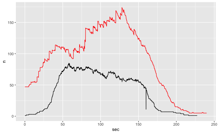
4.7.2 Divided
flow_div_comp = list()
for (i in 1:length(gcs_flow_div_plots)) {
  flow_div_comp[[i]] = gcs_flow_div_plots[[i]] +
  ggplot2::geom_line(data = jps_joined_grouped[[i]],
                     color = "red")
}

gridExtra::grid.arrange(flow_div_comp[[1]], flow_div_comp[[2]],flow_div_comp[[3]],flow_div_comp[[4]], layout_matrix = rbind(c(1,2),c(3,4)))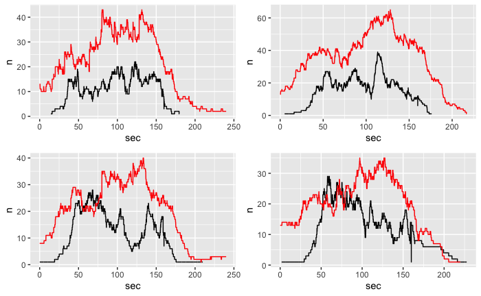
4.7.3 Selected
flow_sel_comp = list()
for (i in 1:length(gcs_flow_zones_plots)) {
flow_sel_comp[[i]] = gcs_flow_zones_plots[[i]] +
ggplot2::geom_line(data = jps_joined_grouped_zones[[i]],
color = "red")
}
gridExtra::grid.arrange(flow_sel_comp[[1]], flow_sel_comp[[2]], layout_matrix = rbind(c(1,2)))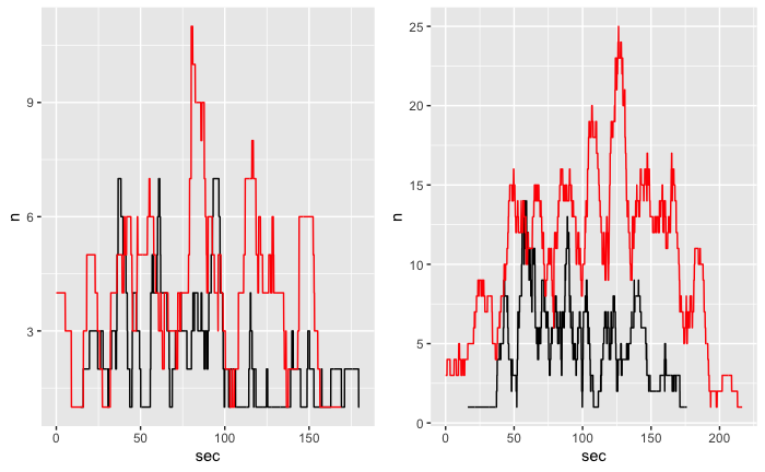 ## Discussion
JPS model (simulated data) has higher flow rate compared to GCS (real data) in all plots. A potential reason for this is that in the JPS model new agents are “injected” into the environement at defined periods of time, which might not be representative of the actual pedestrian dynamics in the concourse. In other words, it is likely that in the real life pedestrians enter and exit the environment based on the train schedule, thus ensuring more or less stable in and out-flow rates. This might not be captured in the model, thus resulting in a peak that is not present in the GCS data.
Importantly, however, we can see that in the plots representing the flow in the selected areas (Zone 1 and 2) the rate is what was expected: Zone 1 is has lower agent flow compared to Zone 2. In this respect the JPS model seems pretty well calibrated even if, in tota, it has higher flow rate.