5 Density

Density measure is similar to flow, but instead of counting the number of agents passing through, for instance, gates, persons per area are measured. Thus, its function is:

Density = N / m2

N = number of agents

Steffen and Seyfried (2010) identify two issues with this density measure:

“in” and “out” of an agent has to be assigned arbitrarily (p. 1903)
density is dependent on time and placement of a measure area, which might result in “jumps for small area.” (p. 1903)

To address these issues, authors suggest implementing Voronoi diagrams. This will be done in the “Voronoi” chapter of this report.

Before moving on, I assume that density plots will resemble flow plots as both of them rely on the number of agents passing through a given area/line, but in density measure the flow rate is divided by an area (m2) of a measured area. Theoretically, if an area is 1m2x1m2 then the flow and density plots would overlap.

5.1 1.1 Global (GCS)

# group by seconds and then measure density
gcs_d = gcs_sf |> 
  sf::st_drop_geometry() |> 
  dplyr::mutate(sec = as.numeric(frame)/25) |>  # 1 sec = 25 frames
  dplyr::group_by(sec) |> 
  dplyr::summarise(n = dplyr::n(),
                   frame = frame) |> 
  dplyr::mutate(
    density = n / gcs_area 
  )

gcs_d |> head()

5.1.1 Plotting

gcs_density = ggplot2::ggplot(gcs_d)+
  ggplot2::aes(x = sec,
               y = density)+
  ggplot2::geom_line()

print(gcs_density)

Density plot looks exactly the same as flow plot.

ggplot2::ggplot(gcs_d)+
  ggplot2::aes(x = sec,
               y = density)+
  ggplot2::geom_line() +
  ggplot2::geom_line(data = gcs_d,
                     ggplot2::aes(x = sec,
                                  y = n),
                     col = "red")

5.2 1.2 Divided GCS density

# add area as a new column
gcs_den_div = list()
for (i in 1:length(gcs_joined_grouped)){
  gcs_den_div[[i]] = gcs_joined_grouped[[i]] |> dplyr::mutate(area = gcs_area_div[i])
}

# find density for each group in each list
gcs_d_div = list()
for (i in 1:length(gcs_area_div)){
  gcs_d_div[[i]] = gcs_den_div[[i]] |> dplyr::mutate(density = n / gcs_area_div[i])
}

5.2.1 Plotting

gcs_den_plots = list()
for (i in 1:length(gcs_d_div)){
  gcs_den_plots[[i]] = ggplot2::ggplot(gcs_d_div[[i]]) +
    ggplot2::aes(x = sec,
                 y = density) +
    ggplot2::geom_line() 
}

# let's plot a polygons 1-4 and 5-8
gridExtra::grid.arrange(gcs_den_plots[[1]], gcs_den_plots[[2]], gcs_den_plots[[3]], gcs_den_plots[[4]], layout_matrix = rbind(c(1,2),c(3,4)))

5.3 1.3 Selected (GCS)

# add area as a new column
gcs_den_sel = list()
for (i in 1:length(gcs_joined_zones)){
  gcs_den_sel[[i]] = gcs_joined_grouped_zones[[i]] |> dplyr::mutate(area = gcs_area_sel[i])
}

# find density for each group in each list
gcs_d_sel = list()
for (i in 1:length(gcs_joined_zones)){
  gcs_d_sel[[i]] = gcs_den_sel[[i]] |> dplyr::mutate(density = n / gcs_area_sel[i])
}

5.3.1 Plotting

gcs_den_sel_plots = list()
for (i in 1:length(gcs_d_sel)){
  gcs_den_sel_plots[[i]] = ggplot2::ggplot(gcs_d_sel[[i]]) +
    ggplot2::aes(x = sec,
                 y = density) +
    ggplot2::geom_line() 
}

# let's plot a polygons 1-4 and 5-8
gridExtra::grid.arrange(gcs_den_sel_plots[[1]], gcs_den_sel_plots[[2]], layout_matrix = rbind(c(1,2)))

5.4 2.1 Global (JPS)

# group by seconds and then measure density
jps_d = traj1_sf |> 
  sf::st_drop_geometry() |> 
  dplyr::mutate(sec = FR/25) |>  # 1 sec = 25 frames
  dplyr::group_by(sec) |> 
  dplyr::summarise(n = dplyr::n(),
                   sec = sec) |> 
  dplyr::mutate(
    density = n / gcs_area
  )

5.4.1 Plotting

jps_density = ggplot2::ggplot(jps_d)+
  ggplot2::aes(x = sec,
               y = density)+
  ggplot2::geom_line()

print(jps_density)

5.5 2.2 Divided (JPS)

# add area as a new column
jps_den_div = list()
for (i in 1:length(jps_joined_grouped)){
  jps_den_div[[i]] = jps_joined_grouped[[i]] |> dplyr::mutate(area = gcs_area_div[i])
}

# find density for each group in each list
jps_d_div = list()
for (i in 1:length(gcs_area_div)){
  jps_d_div[[i]] = jps_den_div[[i]] |> dplyr::mutate(density = n / gcs_area_div[i])
}

5.5.1 Plotting

jps_den_div_plots = list()
for (i in 1:length(jps_d_div)){
  jps_den_div_plots[[i]] = ggplot2::ggplot(jps_d_div[[i]]) +
    ggplot2::aes(x = sec,
                 y = density) +
    ggplot2::geom_line() 
}

# let's plot a polygons 1-4 
gridExtra::grid.arrange(jps_den_div_plots[[1]], jps_den_div_plots[[2]], jps_den_div_plots[[3]], jps_den_div_plots[[4]], layout_matrix = rbind(c(1,2),c(3,4)))

5.6 2.3 Selected (JPS)

# add area as a new column
jps_den_sel = list()
for (i in 1:length(jps_joined_zones)){
  jps_den_sel[[i]] = jps_joined_grouped_zones[[i]] |> dplyr::mutate(area = gcs_area_sel[i])
}

# find density for each group in each list
jps_d_sel = list()
for (i in 1:length(jps_joined_zones)){
  jps_d_sel[[i]] = jps_den_sel[[i]] |> dplyr::mutate(density = n / gcs_area_sel[i])
}

5.6.1 Plotting

jps_den_sel_plots = list()
for (i in 1:length(jps_d_sel)){
  jps_den_sel_plots[[i]] = ggplot2::ggplot(jps_d_sel[[i]]) +
    ggplot2::aes(x = sec,
                 y = density) +
    ggplot2::geom_line() 
}

# let's plot a polygons 1-4 
gridExtra::grid.arrange(jps_den_sel_plots[[1]], jps_den_sel_plots[[2]], layout_matrix = rbind(c(1,2)))

5.7 Comparison

5.7.1 Global

density_comp = gcs_density + 
  # ggplot2::ggplot(jps_grouped) +
  ggplot2::geom_line(data = jps_d,
                     color = "red")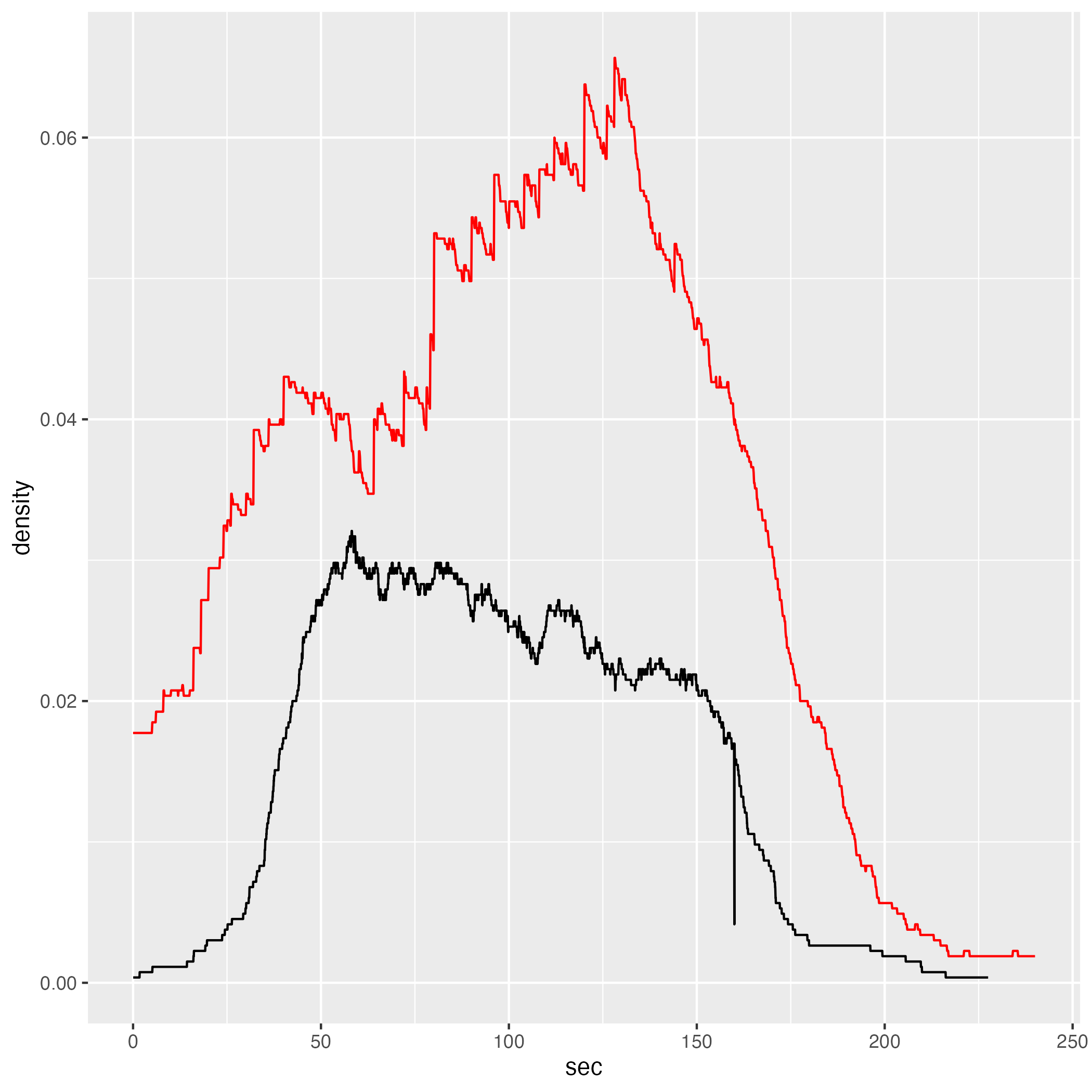

print("GCS mean density value")
gcs_d |> dplyr::group_by(sec) |> dplyr::pull(density) |> mean()
print("JPS mean density value")
jps_d |> dplyr::group_by(sec) |> dplyr::pull(density) |> mean()

print("GCS median density value")
gcs_d |> dplyr::group_by(sec) |> dplyr::pull(density) |> median()
print("JPS median density value")
jps_d |> dplyr::group_by(sec) |> dplyr::pull(density) |> median()

[1] “GCS mean density value” [1] 0.02354127

[1] “JPS mean density value” [1] 0.04464389

[1] “GCS median density value” [1] 0.02566038

[1] “JPS median density value” [1] 0.04566038

5.7.2 Divided

density_div_comp = list()
for (i in 1:length(gcs_den_div_plots)) {
  density_div_comp[[i]] = gcs_den_div_plots[[i]] + 
  ggplot2::geom_line(data = jps_d_div[[i]],
                     color = "red")
}

gridExtra::grid.arrange(density_div_comp[[1]], density_div_comp[[2]], density_div_comp[[3]], density_div_comp[[4]], layout_matrix = rbind(c(1,2),c(3,4)))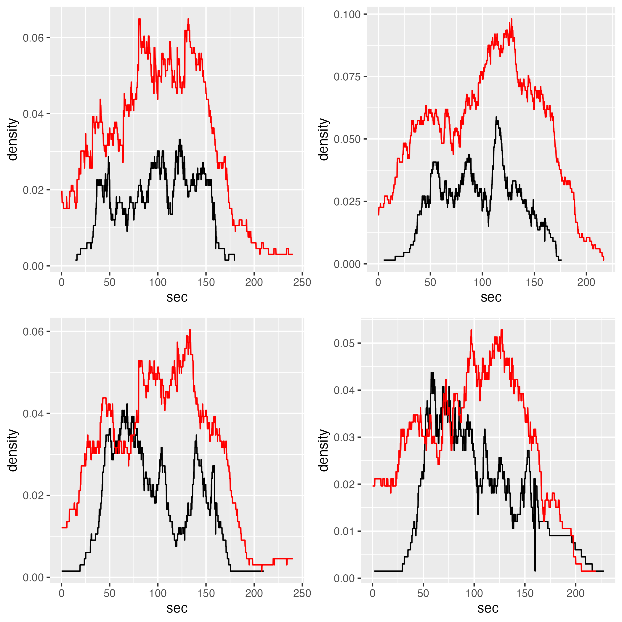

5.7.3 Selected

flow_sel_comp = list()
for (i in 1:length(gcs_flow_zones_plots)) {
  flow_sel_comp[[i]] = gcs_flow_zones_plots[[i]] + 
  ggplot2::geom_line(data = jps_joined_grouped_zones[[i]],
                     color = "red")
}

gridExtra::grid.arrange(flow_sel_comp[[1]], flow_sel_comp[[2]], layout_matrix = rbind(c(1,2)))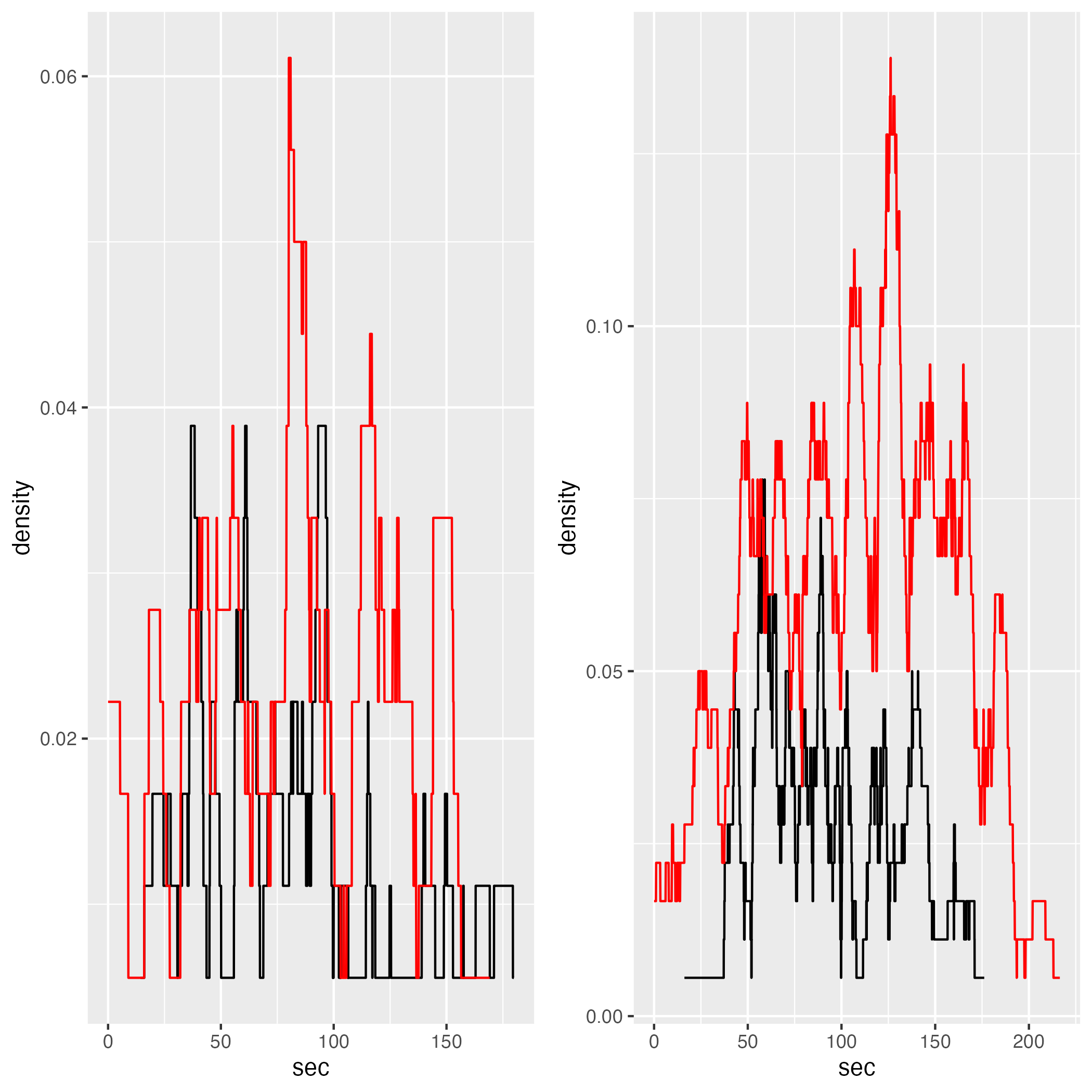

6 Discussion

Since, as mentioned in the introduction of this chapter, flow and density measures are similar, I will not discuss the potential reasons of different densities. Instead, I’d like to note that even in JPS model, which shows higher agent density compared to GCS, the actual density is still relatively low. For instance, in Zone 2 the density is, mostly, below 0.1 person/m2.

Low density, we may assume, does not create conditions for congestion, which is often a subject in the literature of pedestrian dynamics. Therefore, neither in GCS nor in JPS models agents are expected to slow down as the density increases because it does not become dense enough as to cause crowding.

To explore the relationship between density and speed, we will plot fundamental diagrams in the next chapter.