# average speed per frame
gcs_speed1 = gcs_sf_s |>
  dplyr::group_by(sec) |>
  dplyr::summarise(n = dplyr::n())
gcs_speed2 = gcs_sf_s |>
  dplyr::mutate(dist = as.numeric(dist)) |>
  dplyr::filter(dist != 0) |> # filter our starting points (ie the rows that have dist = 0)
  dplyr::group_by(sec) |>
  dplyr::summarise(dist_sum = sum(dist)) |>  # summing up the total distance of agents in a group
  sf::st_drop_geometry() # drop geometry column
gcs_speed = dplyr::left_join(gcs_speed1, gcs_speed2) |>
  dplyr::mutate(speed_av = dist_sum/n) # average speed (see formula at the start of the notebook)
gcs_speed_joined = dplyr::left_join(gcs_speed, gcs_d)7 Fundamental diagrams
The aim of this chapter is to plot fundamental diagrams (speed ~ density) and compare them between JPS and GCS.
A fundamental diagram denotes to the linear relationship between average speed (or velocity) and density (or flow) of an agent, usually vehicles or pedestrians.
Density = N/Area
Speed(av) = sum(agent distance per frame)/N
N = number of agents
Area = an area in which agents are counted
It should be noted that fundamental diagrams may be slightly influenced by different measurement methods (Zhang et al., 2011). However, the aim of this chapter is not to compare different methods but rather understand the extent to which simulated (JPS) data reflects real-life GCS data. Therefore, the focus in this chapter is on classical density and average speed.
The feature of a fundamental diagram is that with “growing density, the velocity decreases monotonically” (Helbing, 2001: sec B, para 3). In other words, the agent speed decreases when an area becomes crowded.
Thus, the traditional hypothesis would be that in both GCS and JPS models the agent speed decreases as the environment becomes more populated. However, given low densities in both environments (show in “Density” chapter) allows to hypothesize that pedestrians would not show a decrease in speed simply because the environment does not become dense enough.
Note 1: GCS has distance/speed per frame data. You can find out how it was acquired following this R script: https://github.com/GretaTimaite/pedestrian_simulation/blob/main/gcs_speed.R
7.1 1.1 Global (GCS)
This builds on the previous chapter on density, hence density part will be skipped. Instead, let’s move to finding out average speed per frame.
7.2 Plotting
gcs_fd = ggplot2::ggplot(data = gcs_speed_joined,
                ggplot2::aes(x = density,
                            y = speed_av))+
  ggplot2::geom_point()
7.3 1.2 Divided (GCS)
To find out how density has been measured, see “Density” chapter.
# first create a list to store our new datasets
gcs_fd_div = list()
for (i in 1:lengths(gcs_div_sf)){
  gcs_fd_div[[i]] = gcs_sf_s[gcs_div_sf[i,], op = sf::st_intersects]
}
# a list with dataframes (denoting to different polygons) containing average speed of agents per frame
gcs_speed_div = list()
for (i in 1:lengths(gcs_div_sf)){
gcs_speed_div[[i]] = gcs_fd_div[[i]] |>
dplyr::mutate(dist = as.numeric(dist)) |> # turn character into numeric
dplyr::filter(dist != 0) |> # filter out agent starting points (eg distance = 0)
dplyr::group_by(sec) |>
dplyr::summarise(n = dplyr::n(), # number of agents per frame
dist_sum = sum(dist), # total sum
speed_av = dist_sum / n) # average speed
}# join dataframes in `gcs_speed_div` and `gcs_speed_div` lists accordingly (will help when plotting)
gcs_fd_joined = list()
for (i in 1:length(gcs_fd_div)){
gcs_fd_joined[[i]] = dplyr::left_join(gcs_speed_div[[i]] |> sf::st_drop_geometry(),
gcs_d_div[[i]] |> sf::st_drop_geometry())
}7.3.1 Plotting
gcs_div_plots = list()
for (i in 1:length(gcs_fd_joined)){
  gcs_div_plots[[i]] = ggplot2::ggplot(gcs_fd_joined[[i]]) +
    ggplot2::aes(x = density,
                 y = speed_av) +
    ggplot2::geom_point()
  # print(plots_den)
}
gridExtra::grid.arrange(gcs_div_plots[[1]], gcs_div_plots[[2]], gcs_div_plots[[3]], gcs_div_plots[[4]], layout_matrix = rbind(c(1,2),c(3,4)))
7.4 1.3 Selected (GCS)
# first create a list to store our new datasets
gcs_fd_sel = list()
for (i in 1:length(zones)){
  gcs_fd_sel[[i]] = gcs_sf_s[gcs_div_sf[i,], op = sf::st_intersects]
}
# a list with dataframes (denoting to different polygons) containing average speed of agents per frame
gcs_speed_sel = list()
for (i in 1:lengths(zones)){
jps_speed_sel[[i]] = gcs_fd_sel[[i]] |>
dplyr::mutate(dist = as.numeric(dist)) |> # turn character into numeric
dplyr::filter(dist != 0) |> # filter out agent starting points (eg distance = 0)
dplyr::group_by(sec) |>
dplyr::summarise(n = dplyr::n(), # number of agents per frame
dist_sum = sum(dist), # total sum
speed_av = dist_sum / n) # average speed
}# join lists accordingly (will help when plotting)
gcs_fd_joined = list()
for (i in 1:length(zones)){
gcs_fd_joined[[i]] = dplyr::left_join(gcs_speed_div[[i]] |> sf::st_drop_geometry(),
gcs_d_div[[i]] |> sf::st_drop_geometry())
}7.4.1 Plotting
gcs_sel_plots = list()
for (i in 1:length(gcs_fd_joined)){
  gcs_sel_plots[[i]] = ggplot2::ggplot(gcs_fd_joined[[i]]) +
    ggplot2::aes(x = density,
                 y = speed_av) +
    ggplot2::geom_point()
  # print(plots_den)
}

gridExtra::grid.arrange(gcs_sel_plots[[1]], gcs_sel_plots[[2]], layout_matrix = rbind(c(1,2)))
7.5 2.1 Global (JPS)
We don’t have dist column in our traj1 dataframe. Thus, we will need to derive it. We will measure speed per secon.
This builds on the previous chapter on density, hence density part will be skipped. Instead, let’s move to finding out average speed per second.
# average speed per frame
jps_speed1 = jps_dist_df |>
  dplyr::mutate(sec = FR / 8) |>
  dplyr::group_by(sec) |>
  dplyr::summarise(n = dplyr::n(),
                   FR = FR,
                   ID = ID)
jps_speed2 = jps_dist_df |>
  sf::st_drop_geometry() |> # drop geometry column
  dplyr::mutate(sec = FR / 8) |>
  dplyr::mutate(dist = as.numeric(dist)) |>
  dplyr::filter(dist != 0) |> # filter our starting points (ie the rows that have dist = 0)
  dplyr::group_by(sec) |>
  dplyr::summarise(dist_sum = sum(dist),
                   FR = FR,
                   ID = ID)   # summing up the total distance of agents in a group
jps_speed = dplyr::left_join(jps_speed1, jps_speed2) |>
  dplyr::mutate(speed_av = dist_sum/n) # average speed (see formula at the start of the notebook)

jps_d_group_sec = jps_d |>
  dplyr::group_by(sec) |>
  dplyr::summarise(n = dplyr::n(),
                   density = density)
jps_speed_joined = dplyr::left_join(jps_speed, jps_d_group_sec)
7.6 Plotting
jps_fd = ggplot2::ggplot(data = jps_speed_joined,
                ggplot2::aes(x = density,
                            y = speed_av))+
  ggplot2::geom_point()
7.7 Divided (JPS)
To find out how density has been measured, see “Density” chapter.
# first create a list to store our new datasets

# turn df into an sf object
jps_dist_sf = jps_dist_df |>
  sf::st_as_sf(coords = c("x_coord", "y_coord"))

jps_fd_div = list()
for (i in 1:lengths(gcs_div_sf)){
  jps_fd_div[[i]] = jps_dist_sf[gcs_div_sf[i,], op = sf::st_intersects]
}
# a list with dataframes (denoting to different polygons) containing average speed of agents per frame
jps_speed_div = list()
for (i in 1:lengths(gcs_div_sf)){
jps_speed_div[[i]] = jps_fd_div[[i]] |>
dplyr::mutate(sec = FR / 8) |>
dplyr::mutate(dist = as.numeric(dist)) |> # turn character into numeric
dplyr::filter(dist != 0) |> # filter out agent starting points (eg distance = 0)
dplyr::group_by(sec) |>
dplyr::summarise(n = dplyr::n(), # number of agents per frame
dist_sum = sum(dist), # total sum
speed_av = dist_sum / n) # average speed
}# join dataframes in `gcs_speed_div` and `gcs_speed_div` lists accordingly (will help when plotting)
jps_fd_joined = list()
for (i in 1:length(jps_fd_div)){
jps_fd_joined[[i]] = dplyr::left_join(jps_speed_div[[i]] |> sf::st_drop_geometry(),
jps_d_div[[i]] |> sf::st_drop_geometry())
}7.7.1 Plotting
jps_div_plots = list()
for (i in 1:length(jps_fd_joined)){
  jps_div_plots[[i]] = ggplot2::ggplot(jps_fd_joined[[i]]) +
    ggplot2::aes(x = density,
                 y = speed_av) +
    ggplot2::geom_point()
  # print(plots_den)
}
gridExtra::grid.arrange(jps_div_plots[[1]], jps_div_plots[[2]], jps_div_plots[[3]], jps_div_plots[[4]], layout_matrix = rbind(c(1,2),c(3,4)))
7.8 Selected (JPS)
# first create a list to store our new datasets
jps_fd_sel = list()
for (i in 1:length(zones)){
  jps_fd_sel[[i]] = jps_dist_sf[zones[i], op = sf::st_intersects]
}
# a list with dataframes (denoting to different polygons) containing average speed of agents per frame
jps_speed_sel = list()
for (i in 1:length(zones)){
jps_speed_sel[[i]] = jps_fd_sel[[i]] |>
dplyr::mutate(sec = FR / 8) |>
dplyr::mutate(dist = as.numeric(dist)) |> # turn character into numeric
dplyr::filter(dist != 0) |> # filter out agent starting points (eg distance = 0)
dplyr::group_by(sec) |>
dplyr::summarise(n = dplyr::n(), # number of agents per frame
dist_sum = sum(dist), # total sum
speed_av = dist_sum / n) # average speed
}# join lists accordingly (will help when plotting)
jps_fd_joined = list()
for (i in 1:length(zones)){
jps_fd_joined[[i]] = dplyr::left_join(jps_speed_sel[[i]] |> sf::st_drop_geometry(),
jps_d_sel[[i]] |> sf::st_drop_geometry())
}7.8.1 Plotting
jps_sel_plots = list()
for (i in 1:length(jps_fd_joined)){
  jps_sel_plots[[i]] = ggplot2::ggplot(jps_fd_joined[[i]]) +
    ggplot2::aes(x = density,
                 y = speed_av) +
    ggplot2::geom_point()
  # print(plots_den)
}

gridExtra::grid.arrange(jps_sel_plots[[1]], jps_sel_plots[[2]], layout_matrix = rbind(c(1,2)))
8 Comparison
8.1 Global
#fd_comp = gcs_fd +
  ggplot2::geom_point(data = jps_speed_joined,
                      color = "red")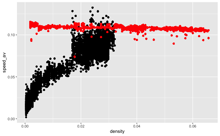
8.2 Divided
fd_div_comp = list()
for (i in 1:length(gcs_fd_div)) {
  fd_div_comp[[i]] = gcs_div_plots[[i]] +
  ggplot2::geom_point(data = jps_fd_joined[[i]],
                     color = "red")
}

gridExtra::grid.arrange(fd_div_comp[[1]], fd_div_comp[[2]], fd_div_comp[[3]], fd_div_comp[[4]], layout_matrix = rbind(c(1,2),c(3,4)))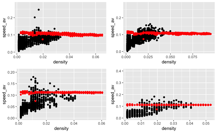
8.3 Selected
gcs_fd_div_plots+
  ggplot2::geom_point(data = jps_fd_joined,
                      color = "red")


fd_sel_comp = list()
for (i in 1:length(gcs_fd_div_plots)) {
  fd_sel_comp[[i]] = gcs_fd_div_plots[[i]] +
  ggplot2::geom_point(data = jps_fd_joined[[i]],
                     color = "red")
}

gridExtra::grid.arrange(fd_sel_comp[[1]], fd_sel_comp[[2]], layout_matrix = rbind(c(1,2),c(3,4)))
9 Discussion
Fundamental diagrams do not show the expected negative slope – the increase in density does not lead to a decreased speed. Indeed, a reverse pattern can be seen in all GCS plots. Arguably, this is a case because in all areas the density remains low enough not to reduce agent speed. An increase in average speed and density might be a result of a new agent entering the area that walks fast, thus boosting the av.speed and density (a little bit!).
In case of JPS, we can observe a steady relationship between speed and density. Again, it is likely that the environment does not become crowded enough to force agents to stop and slow down. Moreover, in the JPS agent speed is set (i.e. is constant), thus reducing the variance of agent speeds. This, however, does not represent the actual pedestrian dynamics in the GCS in which pedestrians might randomly stop to check, for instance, their phones or speed up or slow down depending on their individual circumstances (e.g. how much time is left before train departure).
What could be done next?
- In this example I relied on classical density measure but there are other ways to measure it. For example, Duives et al. (2015) discuss 7 measures for quantifying pedestrian crowdedness in which Voronoi and X-T measures are considered “the best”. It could be useful to explore different methods to confirm (or not) that the negative slope remains in GCS and the current JPS models.
- Plot speed~voronoi density
- Aggregate frames into seconds (ie 25 frames for GCS and 8 frames for JPS)
- It could be interesting to experiment with different agent numbers in JPS to explore when/how congestion occurs, thus leading to the expected outcome – as density increases, speed/velocity decreases.